2. Adding arbitrary curves and removing default curves
Adjusting defaults
The region constructors provide default settings that can be modified by keyword argument. Try turning on/off the default boundary lines, lines of constant radius, and (u,v) coordinate (null Eddington-Finklestein) grid:
import xhorizon as xh
import matplotlib.pyplot as plt

f = xh.mf.reissner_nordstrom(M=0.5, Q=0.3)

reg = xh.reg.MAXreg(f, boundary=True, rlines=False, uvgrid=False)

xh.newfig()
reg.rplot()
plt.savefig("out.png")
To start from a blank canvas set all three keywords False. Then you can add whatever curves you like to the diagram.
Adding arbitrary curves manually
As a test case let’s add the rather arbitrary curve
defined in Schwarzschild coordinates, into a Schwarzschild diagram:
import xhorizon as xh
import numpy as np
import matplotlib.pyplot as plt

f = xh.mf.schwarzschild(R=1)
reg = xh.reg.MAXreg(f, boundary=True, rlines=False, uvgrid=False)

t = np.linspace(-50,50,1001)
r = 1.5 + 0.25*np.sin(t)

crv = xh.curve()
crv.tr = np.array([t,r])
crv.sty = dict(c='magenta', lw=1, zorder=0)

for b in reg.blocks:
    b.add_curves_tr([crv])

xh.newfig(sqaxis=2)
reg.rplot()
plt.savefig("out.png")
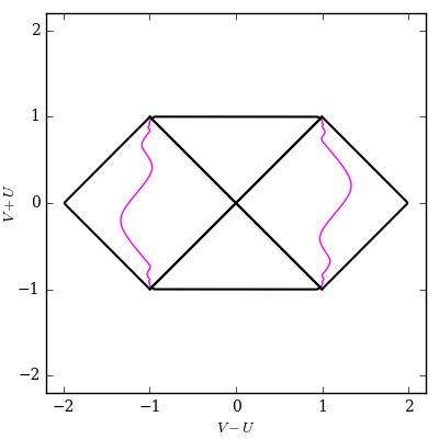
The command xh.curve() created a “curve” object. A curve object represents the same curve in various coordinate systems. In this case we create the curve with Schwarzschild (t,r) coordinates only. Later, when b.add_curves_tr() is called, the region object automatically performs coordinate transformations to fill in other coordinate representations of the curve.
You will notice there are two copies of the curve.
This is because a region actually consists of a collection of blocks. Each block has its own patch of Schwarzschild (t,r) and Eddington-Finklestein (u,v) coordinates. Blocks are separated by horizons (where \(f(r)=0\)) and bounded by \(r=0\) and \(r=\infty\). These separations/boundaries are, of course, precisely where patches of Schwarzschild coordinates end.
With the loop for b in reg.blocks we attempted to add the curve to every block in the region. However, the function block.add_curves_tr() rejects curves that include invalid radii for the block. In this case the curve lies entirely outside the horizon at \(R=2M=1\), and is successfully added to both “exterior” (\(r>R\)) blocks.
You can also add curves in \((u,v)\) coordinates, or equivalently \((t,r_{*})\) coordinates, with b.add_curves_uv(). You can also add curves only to specific blocks. Both shown below.
Note that the argument of block.add_curves_tr() is a list of curves. Here we only created one curve, so the argument was a length-one list crvlist = [crv]. More generally we can input a list of curve objects like [crv1,crv2] to add many curves at once. In the source this is often done by initiating a list crvlist = [] and iterating through things of the form crvlist += [crv] to extend the list inside of a loop, then calling block.add_curves_tr(crvlist). The same goes for block.add_curves_uv() and related functions.
Add curves to specific blocks
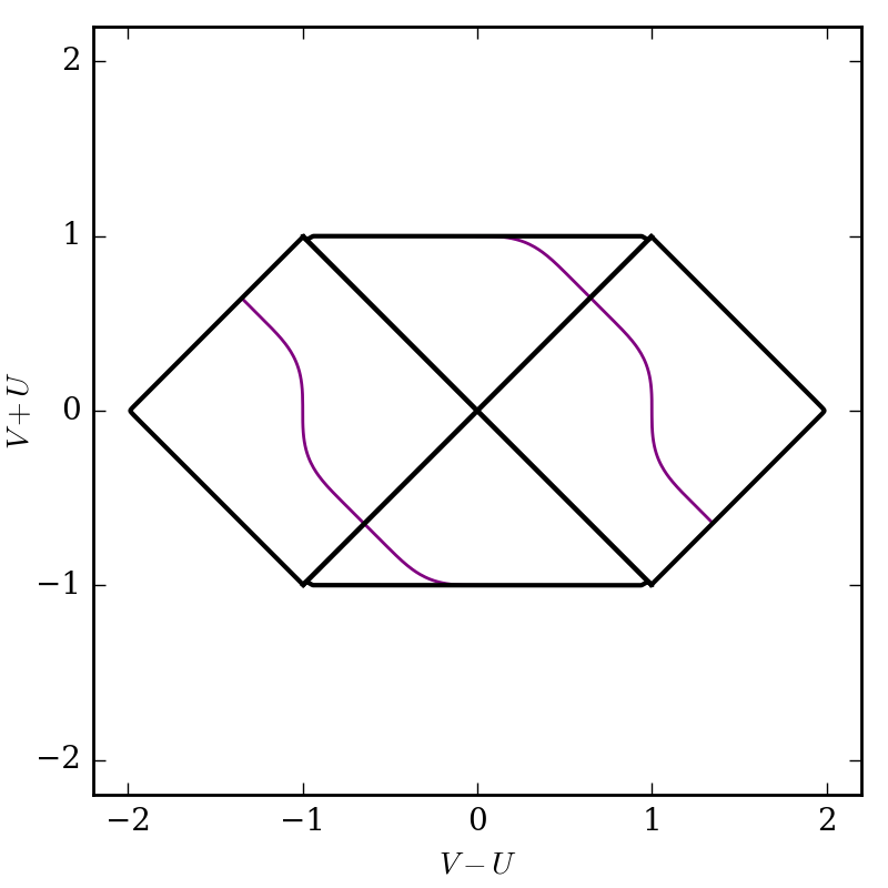
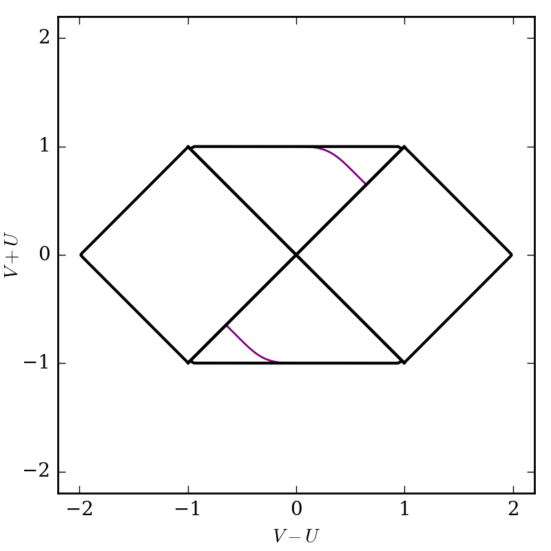
Suppose we want to add a curve only to certain blocks. Let’s consider the curve, defined in Eddington-Finklestein coordinates,
that is valid in any block.
Adding to all blocks as before we have:
import xhorizon as xh
import numpy as np
import matplotlib.pyplot as plt

f = xh.mf.schwarzschild(R=1)
reg = xh.reg.MAXreg(f, boundary=True, rlines=False, uvgrid=False)

u = np.linspace(-50,50,1001)
v = np.tanh(u)

crv = xh.curve()
crv.uv = np.array([u,v])
crv.sty = dict(c='purple', lw=1, zorder=0)

for b in reg.blocks:
    b.add_curves_uv([crv])

xh.newfig(sqaxis=2)
reg.rplot()
plt.savefig("out.png", dpi=200)
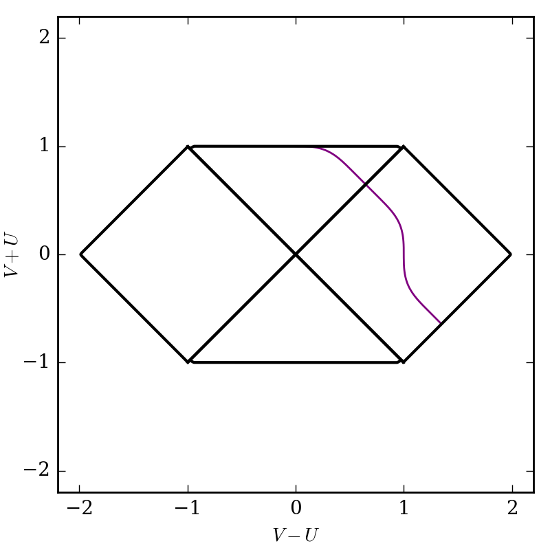
To choose specific blocks to add the curve to, you can select them manually (find correct indices by guess and check):
import xhorizon as xh
import numpy as np
import matplotlib.pyplot as plt

f = xh.mf.schwarzschild(R=1)
reg = xh.reg.MAXreg(f, boundary=True, rlines=False, uvgrid=False)

u = np.linspace(-50,50,1001)
v = np.tanh(u)

crv = xh.curve()
crv.uv = np.array([u,v])
crv.sty = dict(c='purple', lw=1, zorder=0)

reg.blocks[0].add_curves_uv([crv])
reg.blocks[1].add_curves_uv([crv])

xh.newfig(sqaxis=2)
reg.rplot()
plt.savefig("out.png", dpi=200)
Alternately perhaps you only want to add curves to the “interior” or “exterior” blocks. Blocks contain an integer parameter block.j which describes which radius interval they are in. The case j=0 is the innermost block, bounded by \(r=0\) and the innermost horizon radius. Each subsequent index moves radially outward. In the Schwarzschild case there is one horizon so the only options are j=0 and j=1. Here to plot only in interior blocks we could do:
import xhorizon as xh
import numpy as np
import matplotlib.pyplot as plt

f = xh.mf.schwarzschild(R=1)
reg = xh.reg.MAXreg(f, boundary=True, rlines=False, uvgrid=False)

u = np.linspace(-50,50,1001)
v = np.tanh(u)

crv = xh.curve()
crv.uv = np.array([u,v])
crv.sty = dict(c='purple', lw=1, zorder=0)

for b in reg.blocks:
    if b.j==0:
        b.add_curves_uv([crv])

xh.newfig(sqaxis=2)
reg.rplot()
plt.savefig("out.png", dpi=200)
Curve stylings
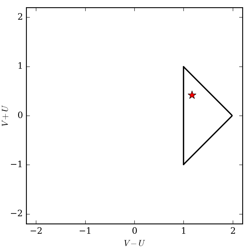
Note that the style field curve.sty is a dictionary of parameters to be passed along to plt.plot(), any of its keyword arguments should work. You can use this to specify linestyles, markers, widths, colors, etc. To plot specific points use a curve with just one point and set a marker:
import xhorizon as xh
import numpy as np
import matplotlib.pyplot as plt

f = xh.mf.minkowski()
reg = xh.reg.MAXreg(f, boundary=True, rlines=False, uvgrid=False)

t = np.array([1.75])
r = np.array([0.91])

crv = xh.curve()
crv.tr = np.array([t,r])
crv.sty = dict(c='red', marker='*', markersize=10, zorder=0)

reg.blocks[0].add_curves_tr([crv])

xh.newfig(sqaxis=2)
reg.rplot()
plt.savefig("out.png", dpi=200)
Using built-in curvemakers
…